-
Best Australian Pokies Free No Download No Registration
Poker Tournaments Brisbane Casino
Tips No Deposit Pokies 2024
Deposit Casino Pokies Win Real Money Australia
Australia Casinos That Accept Skrill 2024
Commercial Hotel Werribee Pokies
Try Pokies in Australia Machines for Free
Bingo Bonuses AU
Australian Roulette Online Game
Poker AU Casino
Reinforcement Learning Implicit Stock Trends
*Team final project completed for Harvard’s Artificial Intelligence course, CS 182, together with Ziyi (Queena) Zhou & Julien Laasri*
Overview
Many have tried to analyze the stock market, attempting to pull out a pattern from the frenzy of transactions and capitalize on it. In short, we thought we’d have a go as well by creating an AI agent that could learn from stock history to make profitable decisions. More specifically, the goal of our project was to use reinforcement learning techniques to train agents that can determine the best time to buy/sell a stock within a given time frame.
Stock transactions happen for a select number of hours during the day, and a select number of days in any given week. NASDAQ, as an example, operates from 9:30am to 4:00pm EST during weekdays (barring holidays). Bids and asks turn into trades that happen extremely fast, on a millisecond timescale. Along with pure pricing information, a number of metrics are used to characterize the market, such as the volume of sales, the momentum of the market, etc. (check out 70+ KPI’s here). Unfortunately for us, most of the high resolution price data was locked behind a pay-wall. Therefore, we chose to use Yahoo! Finance as a free source that provides daily prices for a host of companies on the NADAQ market. On any given day, a stock has an associated opening, closing, high and low price. We selected price histories of the following four tech companies:
- Amazon
- Apple
- Microsoft
By evaluating our agents on multiple companies, we are ensuring the agents develop policies that are generalizable. Furthermore, we chose companies within the same industry so as to control for possible discrepancies in long-term or short-term trends between industries. Out of the four companies, Google is the youngest, going public on August 19, 2004. As a result, we restricted our scope to examine prices 2005 onward.
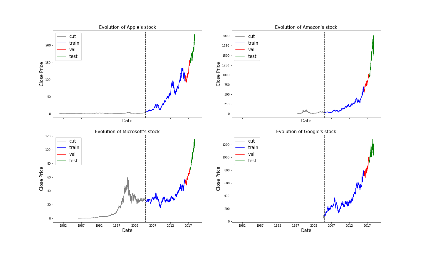
The figure above shows the stock histories of our chosen companies, along with the cut we made to select a consistent time period. We partitioned the remaining data into training, validation, and test sets according to an 80/10/10 split. Next, we dove into the problem specification, outlined in the next section.
Problem Specification
For our project, we chose to implement a binary agent with two possible actions: “buy” and “wait.” The decision to omit the action to sell allows us to define an intuitive problem framework that is easily generalizable to a symmetric agent that can either ”sell” or ”wait.” We define our problem in terms of the following steps:
Split the stock price data into subsets of w days called time windows.
Each day corresponds to a state, in which the agent must make an action (buy or wait). Note that the agent MUST make a purchase within the time window, in order to ensure the agent does not sit idly forever. Also note that the states can include previous days’ trends, dubbed the history, to better inform the agent’s decision.
Once the agent chooses to buy, we skip the remaining days in the current time window and transition to the first state of the next time window.
The reward for the agent’s purchase is based on the amount of money it made/lost within that time window. There is no reward for waiting, but a natural penalty will be incurred if the agent waits past the last day, as the agent will be forced to make a purchase.
These series of steps are represented as a Markov Decision Process (MDP) in the figure below:
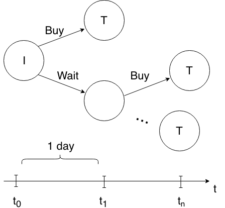
In our MDP, the initial state is marked with an I, while terminal states are marked with T’s. A decision is made on each day, shown on the timeline at the bottom. Note that the timeline represents a single time window.
Agents
The following sections outline the specifics of how we developed our agents within the context of the problem description. We worked on four agents in total. The first is a baseline agent that implements some simple logic to set the standard. The next is an ε-greedy Q-learning agent with a reduced state space. The last two are ε-greedy agents that use approximate Q-learning to predict the Q-values for a continuous state space, one using a linear function, and the other using a neural network.
Baseline
We define a baseline agent that is inspired from the submit and leave (S&L) agent described by Nevmyvaka et al., 2006. The agent has only one constant parameter d. Given a time window, the agent buys the stock only if the price decreases to $d less than the initial price. As all agents have to buy during the time window (by how we defined our MDP), we also force this agent to buy at the last time frame if it does not buy the stock before that.
Exact Q-Learning Agent
Q-learning is the process of iteratively updating the value (called the Q-value) of a (state, action) pair with a function of the rewards obtained from each pass through the tuple. This means that a proper Q-learning framework must reduce the state space so that each (state, action) pair is visited multiple times, otherwise the Q-values will not converge. In order to create a Q-learning agent that fits within the framework of our problem, we abstract away daily prices into daily movements instead. These movements signifies the directionality of the price trend within a particular day, which is the sign of the difference between the close price and the open price. Each state contains h previous movements, corresponding to the desired number of previous days’ trends we wish the agent to consider, as well as the trend of the current day. It is necessary to keep h, the history size, quite small so as not to inflate the size of the state space and risk non-convergence.
Because we lack specific price information within each state, we decide to use a simple reward function that gives a constant positive reward r, for when the agent buys before a price increase the next day (meaning it bought at a low), and consequentially a negative reward −r for when the agent buys before the price dropped the next day (meaning it bought at a high). Unfortunately we are not able to make comparisons to an initial price, and therefore to encourage the agent to buy, instead of forcing the agent to buy within a time window, we give a slight negative reward for choosing to wait −c. However, when evaluating the agents together, we take the actions of the Q-learning agent and evaluate how it would have performed within the context of time windows, even though it is trained to make day to day decisions from historical trends. An example of state representation, the action space, and reward function is summarized below:
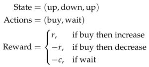
Note that in the example state representation above, h = 2, while the exact significance is: two days ago the price went up, one day ago the price went back down, and today the price went up again.
Approximate Q-Learning: Linear
The benefit of using approximate Q-learning in our problem framework is that we are allowed to have a continuous state space. This is essential because it is very rare that the vector of prices for any given stock on any given day will be the same again in the future. The idea behind approximate Q-learning is that we can predict the Q-values of states given a set of features, f (s, a), which are functions of states s and actions a. Linear function approximation learns weights, w_i, associated with these features, and produces a linear combination of these features as the prediction of the Q-value. In our case, we chose to have each feature be a binary indicator for a (state, action) pair. In other words, we have s · a features, each with an associated weight. This process is formalized through the following equations:

where α corresponds to the learning rate and γ signifies the discount factor.
As before, we include historical information in the states, although this time we are able to include specific prices. Therefore, the state representation is modified to include all four descriptive prices for any given day included in the state. The reward is set to be the negative of the difference in price between the day the agent decides to buy, p_0, and the initial day in the time frame, p_i. The negative sign ensures that positive rewards are allotted for buying at lower prices. An example of state representation, action space and reward function is provided below:
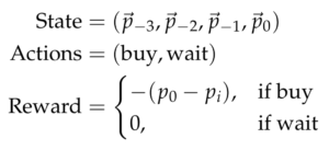
where p_{−3} stands for the vector of prices 3 days ago, p_{−2} is the vector of prices 2 days ago, etc.
Approximate Q-Learning: Deep Neural Network
As in Q-Learning with linear function approximation, deep Q-Learning tries to solve the issue where the state space is continuous and massive. Unlike the linear approximation, deep Q-Learning utilizes a neural network structure to store and approximate the Q-value for a given (state, action) pair. We designed a neural network that takes in inputs s and a, and outputs Q(s, a), using the squared Bellman error to be our loss function:
![]()
Because our action set has a small size, we decided to use two separate neural networks for each action we have. For example, the neural network for action ’buy’ will take s as input and output Q(s, buy). Our deep Q-Learning algorithm comes with some additional hyperparameters:
- The number of hidden layers
- The number of hidden units in each layer
We tuned these two hyperparameters on a hold-out validation set.
Price Prediction
We tried our hand at predicting the next day’s stock price, with the intention to use this as a feature in the state space of our agents to develop better policies. We tried out a handful of machine learning algorithms on a simple 80/20 train/test split on Apple stock data. Altogether, we endeavored to try two different approaches:
Regression
Regression formulation: Can we predict tomorrow’s close price based on today’s information using a linear regression?
To answer this question, we first defined a correct prediction as predicting the close price within an error of at most 2%. Doing so, our model was correct 75.52% of the time on the test set. This seems quite good, but with a deeper investigation we exposed a flaw in the predictions of our model. As shown in the figure below, we only manage to obtain correct predictions when the price doesn’t change much. In the turning points of the price, our predictions tend to be wrong:
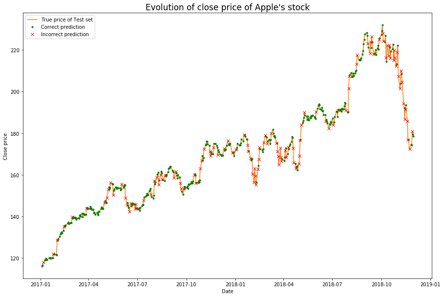
Furthermore, when we zoomed in on our predictions on the test set, we saw that our prediction for the next day was just the price of the current day. We decided to implement a baseline model that would predict tomorrow’s day to be today’s close price. This baseline had a similar performance on the test set, with a prediction accuracy of 76.56%. Unfortunately, this type of prediction would not provide our agents with information they don’t already have, so we decided not to include it in the state space.
Classification
Classification formulation: Can we predict tomorrow’s price movement (up or down) based on 3 previous days’ information, using XGBoost, LightGBM, and Logistic Regression?
Predicting tomorrow’s movement based on the three last days’ information leads to the results in the following table:

As the table shows, the predictions on the test set are close to being random (possibly even worse). The gradient boosting methods, which would be liable to pick up complex nonlinearities, seem to overfit drastically to the training data. The fluctuations of the market seem to be too random for our classification algorithms to capture any real trends that could help us predict even just the movement of the price of future days (perhaps understandably so, otherwise we would have no need for reinforcement learning in the first place). We thus decided to abandon the research on the price prediction algorithms as they did not seem to provide us with valuable information.
Results
Evaluation Strategy
We evaluated our agents by running them on unseen test data without updating the Q-values or the weights they used to predict the Q-values. We then measured the amount of money they were able to make from purchasing at the time they did within the window. We computed this in the same way we computed the reward for the approximate Q-learning agents, by taking the negative of the difference in close price on the day they decide to buy vs. the first day of the time window. This difference of close price was the score that we gave to our agent for that time window. If the agent never decided to buy for that time window, we forced it to buy at the last timestep. We used the validation set to tune the hyperparameters of our agents, and tested all of them on the unseen test set. Our final score was the average score of how our agent performed on all time windows of the unseen test data. We denoted this to be the average profit of our agents.
We realized that there is a lot of variation in the validation scores for models that had the exact same parameters and only a small epsilon value. As such, it became apparent that our agents were not able to converge on a policy. Therefore, we decided to run our scoring regime 51 times for each agent to generate distributions of their average profit for each company as is shown in the figure below:
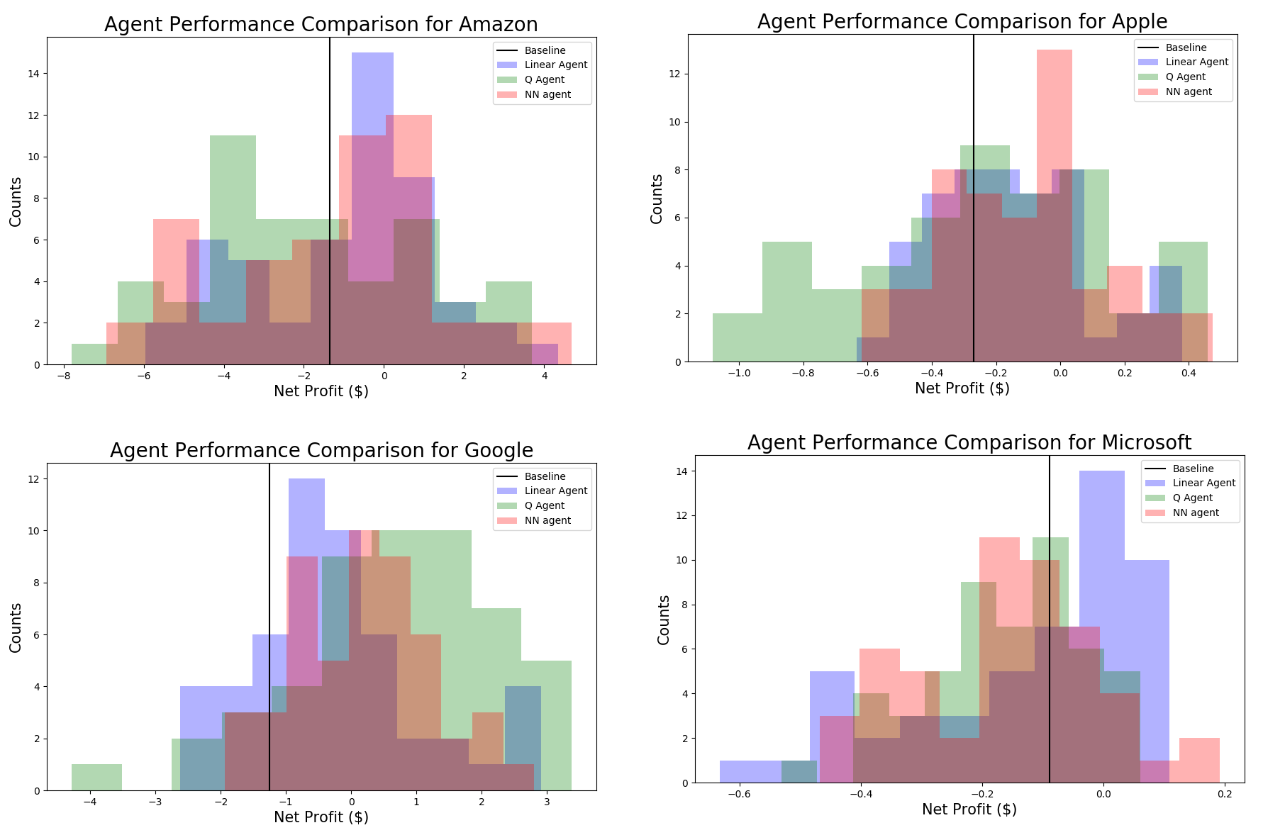
The confidence intervals are Student confidence intervals, our values being considered to be Gaussians with unknown standard deviations.
The performance of each of our agents for each company can be found in the following tables:
- Apple:

- Amazon

- Microsoft


Discussion
The first thing to note from the histograms is that there was a significant spread to the performance of each agent. This is visual confirmation that the agents’ policies did not converge, and therefore they performed differently according to the random fluctuations provided by their ε value. This could be due to several reasons. Firstly, it is possible, as hinted by the price prediction effort, that the stock trends are so random that the agent could not identify any implicit trends in the data. Secondly, we know that there are many external factors that impact stock trends, such as poor publicity, global shortages, company policies, etc. Our agents were ignorant to all of these trends, so what seems like random behavior to them, may be explained by external events. Finally, it is possible that we did not have enough data for our agents to converge on a consistent policy. Our data was relatively low-frequency (daily), as opposed to some of the RL agents we read about that used very high-frequency data (millisecond timescales), of which there is much more to be found.
That being said, we did our best to get a general sense for how the agents performed from our averaging scheme. Looking at the tabular data above, we can see that for each company, the agent that performed the best varies. For Apple, the Deep Learning agent performed the best on average, followed by the linear agent, the Q-learning agent, and then the baseline. This trend follows our expectation, since the Deep Learning agent is most likely to capture nonlinear implicit trends, whereas the others are simpler models, and the order of performance is aligned with the order of simplicity. The company that exhibited characteristics most contrary to the others turned out to be Microsoft, as not only was the standard deviation of the agents’ performances much lower, but the order was nearly reversed, in that the baseline model performed the best on average, as opposed to the RL agents. This could mean that there were subtle effects that confused the agents, whereas the simpler model abstracted away the subtle impacts and gave a better general sense for where the trends were going.
This highlights the strengths and weaknesses of each approach. The strengths of the complex models involve highlighting nonlinear, complex trends within the stock history. This is beneficial when these trends follow a hard to find pattern that repeats itself, but is highly disadvantageous if the patterns do not repeat. In the latter situation, the complex agents are more likely to fit noise, and cannot extrapolate well to the test data. We saw a precursor of this in the price prediction section, when the gradient boosting decision tree methods ended up overfitting the training data dramatically, and were even worse than logistic regression, which was still worse than even randomly guessing.
Another point that we want to highlight is our choice of the time window. We chose the time window to be small enough so that we had more training instances. This was a big tradeoff that we have to balance because it is inherently possible that the agent just had a tough time making decisions within such a short time window. There could be longer effects that don’t manifest themselves on the scales we were searching, or ones that have a periodicity that escaped from our narrow view.
Overall, it appears as though we cannot say for sure whether our agents improved over one another or not, as all of their confidence intervals overlapped. However, we can say that the approximate Q-learning framework allows the agents to capitalize on more information, and therefore at the very least it’s a step in the right direction. Additionally, if we were to make a directional read, in 3/4 of the companies, our approximate learning agents outperformed the baseline on average. In particular, in all four companies, our linear approximation agent outperformed the baseline more than 50% of the time. This is a promising indication.
Conclusion & Future Work
We trained four agents and compared their performance on four technology companies’ stocks. We can see that in certain situations, our three RL agents were able to make greater profits than the baseline agent. This gives us hope that with further tuning, our RL agents could be useful in real life stock market prediction.
In the future, we plan on extending our agents’ state spaces in different ways. First, We could incorporate real financial features used by professionals to lend insight into the state of the market at any given time. Another extension could be to add external data to the state space. As mentioned before, information not available to our agent may directly influence the evolution of the prices of our stocks. As these are currently unknown to our agents, these changes may seem random to them even though they are not. One possibility could be to parse the news related to the company we are interested in and try to spot events that may impact its stocks. A further improvement that we could make would be to revisit the price prediction and try more models that are geared for time series data. We could explore the use of LSTM’s or other types of regression to identify upswings and downswings in the market.
To summarize, we explored various methods for applying reinforcement learning to the stock market with the data we had available. The results were somewhat inconclusive, but there were promising indicators to show that our agents did outperform the baseline in certain situations. We made sure to rigorously and ethically evaluate our agents, and cleaned the data as best we could to ensure their success. We discussed what could have prevented the policies from converging, and also covered several areas for improvement. Identifying trends in the stock market is most definitely a difficult task. Our project elucidated how random the day to day motion of stock prices can be without factoring in external effects or long term trends. Perhaps one day, we can put all our faith in our algorithms. Until then, we shall put our faith in stock brokers.