-
Best Australian Pokies Free No Download No Registration
Poker Tournaments Brisbane Casino
Tips No Deposit Pokies 2024
Deposit Casino Pokies Win Real Money Australia
Australia Casinos That Accept Skrill 2024
Commercial Hotel Werribee Pokies
Try Pokies in Australia Machines for Free
Bingo Bonuses AU
Australian Roulette Online Game
Poker AU Casino
Python Library Development: Automatic Differentiation
*Team final project completed for Harvard’s Systems Development for Computational Science course, CS 207, together with Vincent Viego, Summer Yuan, & Zach Wehrwein*
Overview
NOTE: Install our package with pip install Dotua, and read the How To Use section of the documentation that can be found in the github repo linked above.
The goal of this project was to develop a Python library that can perform automatic differentiation (AD): a computational method for solving derivatives. Before automatic differentiation, computational solutions to derivatives either involved taking finite differences (lacking in precision), or performing symbolic differentiation (lacking in speed). In short, AD provides the best of both worlds, computing derivates extremely quickly and to machine precision.
One incredibly important application of the derivative is optimization. Machines are able to traverse gradients iteratively through calculations of derivatives. However, in machine learning applications, it is possible to have millions of parameters for a given neural network, which leads to a combinatorially onerous number of derivatives to compute analytically. Furthermore, finite difference methods can lead to truncation errors that are orders of magnitude greater than machine precision.
In this webpage we shall provide a background for understanding how AD works, then move on to revealing our library structure and implementation, and finally presenting a few use cases with working examples of the library in action.
As a final note, we chose the name of our package to be Dotua, which is (autoD) backwards.
Automatic Differentiation
The core concept that drives automatic differentiation is the multivariate chain rule. The chain rule states that the derivative of a composition of functions is:
![]()
That is, the derivative is a function of the incremental change in the outer function applied to the inner function, multiplied by the change in the inner function. For instance, if we have a simple function of two variables:
![]()
The total change in y is a function of its partial derivatives with respect to those variables, as well as the changes in u and v, represented as:
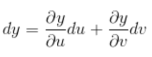
What this example illustrates is that the derivative of a multivariate function can be decomposed into partial derivatives with respect to its sub-functions. The main takeaway here is that in order to solve for the derivative of a complex function, we can propagate the derivatives of the building blocks that were used to construct the complex function we are interested in. Presented more formally, if a machine can compute any given sub-function, as well as the partial derivative between any set of sub-functions, then the machine need only do some simple multiplication and addition to obtain the total derivative.
An intuitive way of understanding automatic differentiation is to think of any complicated function as ultimately a a graph of composite functions. An example that illustrated this is shown below (source):
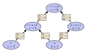
In the graph, each node is a simple operation for which the derivative is readily known, while the edges represent the relationship of change between any two variables, a.k.a, the partial derivatives. To obtain the partial derivative of any single node with respect to any other node, one simply has to sum the paths between any two nodes.
The associative property of derivatives gives rise to two “modes” of forward differentiation: Forward and Reverse. Each has benefits/disadvantages in specific use cases, as will be highlighted further down.
Forward Mode
Within the graph formulation, forward mode automatic differentiation starts with what are known as the seed variable (whatever variable we are taking the derivative with respect to), and keeps track of the derivative through the chain rule as the seed variable is used to build more complex functions. For example, if our seed variable is x, with a seed value of 1 (meaning the derivative with respect to itself is 1), and we define a new function, z = sin(x), our forward mode AD algorithm would automatically update the value of dz/dx using the chain rule to compute dz/dx = d(sin(x))/dx * dx. For our implementation specifically, as we build more complex functions with these elementary operations, we implicitly create a computational graph and solving it as we go. Since all programming languages use a fixed set of elementary functions, we can hardcode these elementary derivatives in order to perform the forward propagation.
One last noteworthy piece to mention is the justification for storing the derivative as an inherent property of the variables we are adding. The justification comes from the notion of dual numbers, numbers that add an extension to real numbers by restating each real number x as x + ε where ε^2 = 0. Dual numbers allow us to track the derivative of even a complicated function, as a kind of data structure that caries both the derivative and ε, the primal of a number. It can be shown that ε encodes the derivative of a variable through the Taylor series expansion of a function:
![]()
When one evaluates f(x+ε) given that ε^2 = 0, then all the higher order terms drop out and we are left with f(x) + f'(x)ε.
Reverse Mode
Reverse mode AD can be understood best when considering the graph and chain rule framework from before. In a nutshell, reverse mode is an inversion of the chain rule, traversing the graph from the “top down” instead of the “bottom up.” Therefore, we start by seeding our final function we wish to evaluate, and then propagate down to the source variables to compute the derivative. In order to achieve this, we store an explicit computational graph, that encodes the connections between functions. In our implementation specifically, this is less space efficient than forward mode, but much more time efficient since we do not have to evaluate the entire computational graph each time the user calls for a partial derivative.
More generally, both forward and reverse mode can be implemented using explicit graphs. With this general framework, consider a situation where the user has a large computational graph with many source variables, but only desires the partial derivative with respect to one. In this case, forward mode would be most efficient since you don’t need to traverse the entire graph. However if you wanted all the partial derivatives, reverse mode would prove more efficient, as you would be able to obtain them all in one go from the top down, whereas in forward mode you’d have to traverse the graph multiple times from the bottom up. Therefore, the two different modes have their tradeoffs depending on the use case.
For more information, Rufflewind has a great article detailing how forward mode and reverse mode automatic differentiation can be implemented in Python.
Implementation
The purpose of the Dotua library is to perform automatic differentiation on user defined functions, where the domain and codomain may be single or multi-dimensional (n.b. this library provides support for both the forward and reverse modes of automatic differentiation, but for the reverse mode only functions with single-dimensional codomains are supported). At a high level, Dotua serves as a partial replacement for NumPy in the sense that Dotua provides methods for many of the mathematical functions
(e.g., trigonometric, inverse trigonometric, hyperbolic, etc.) that NumPy implements; however, while the NumPy versions of these methods can only provide function evaluation, the Dotua equivalents provide both evaluation and differentiation.
To achieve this, the Dotua library implements the following abstract ideas:
- Allowing users to be as expressive as they would like to be by providing
our own versions of binary and unary operators. - Forward AD: keeping track of the value and derivative of user defined
expressions and functions. - Reverse AD: constructing a computational graph from user defined functions
that can be used to quickly compute gradients.
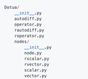
The high level structure of the core of the Dotua library
With these goals in mind the Dotua forward mode implementation relies on the Nodes modules and the Operator class and allows user interface through the AutoDiff class which serves as a Node factory for initializing instances of Scalar and Vector. Analogously, the Dotua reverse mode implementation relies on the Nodes module and the rOperator class and facilitates user interface through the rAutoDiff class which serves as a
factory for initializing instances of rScalar.
Nodes
The Nodes module contains a Node superclass with the following basic design:
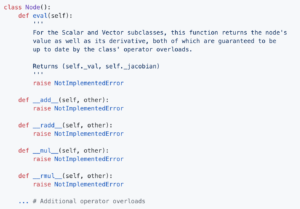
For the Scalar and Vector subclasses, this function returns the node’s value as well as its derivative, both of which are guaranteed to be up to date by the class’ operator overloads.
Essentially, the role of the Node class (which in abstract terms is meant to represent a node in the computational graph underlying forward mode automatic differentiation of user defined expressions) is to serve as an interface for two other classes in the Nodes package: Scalar, Vector, rScalar, rVector. Each of these subclasses implements the required operator overloading as necessary for scalar and vector functions respectively (i.e., addition, multiplication, subtraction, division, power, etc.). This logic is separated into four separate classes to provide increased organization for higher dimensional functions and to allow class methods to use assumptions of specific properties of scalars and vectors to reduce implementation complexity.
Both the Scalar class and the Vector class have _val and _jacobian class attributes which allow for forward automatic differentiation by keeping track of each node’s value and derivative. Both the rScalar class and the rVector class have _roots and _grad_val class attributes which allow for reverse auto differentiation by storing the computational graph and intermediate gradient value.
Scalar
The Scalar class is used for user defined one-dimensional variables. Specifically, users can define functions of scalar variables (i.e., functions defined over multiple scalar variables with a one-dimensional codomain) using instances of Scalar in order to simultaneously calculate the function value and first derivative at a pre-chosen point of evaluation using forward mode automatic differentiation. Objects of the Scalar class are initialized with a value (i.e., the point of evaluation) which is stored in the class attribute self._val (n.b., as the single underscore suggests, this attribute should not be directly accessed or modified by the user). Additionally, Scalar objects – which could be either individual scalar variables or expressions of scalar variables – keep track of their own derivatives in the class attribute self._jacobian. This derivative is implemented as a dictionary with Scalar objects serving as the keys and real numbers as values. Note that each Scalar object’s _jacobian attribute has an entry for all scalar variables which the object might interact with (see AutoDiff Initializer section for more information).
Users interact with Scalar objects in two ways:
- eval(self): This method allows users to obtain the value for a Scalar object at the point of evaluation defined when the user first initialized their Scalar objects. Specifically, this method returns the float self._val.
- partial(self, var): This method allows users to obtain a partial derivative of the given Scalar object with respect to var. If self is one of the Scalar objects directly initialized by the user (see AutoDiff Initializer section), then partial() returns 1 if var == self and 0 otherwise. If self is a Scalar object formed by an expression of other Scalar objects (e.g., self = Scalar(1) + Scalar(2)), then this method returns the correct partial derivative of self with respect to var.
Note that these are the only methods that users should be calling for Scalar objects and that users should not be directly accessing any of the object’s class attributes. Scalar objects support left- and right-sided addition, subtraction, multiplication, division, exponentiation, and negation.
rScalar
The rScalar class is the reverse mode automatic differentiation analog of the Scalar class. That is to say, rScalar is used for user defined one-dimensional variables with which users can define scalar functions (i.e., functions defined over multiple scalar variables with a one-dimensional codomain) in order to calculate the function value and later easily determine the function’s gradient reverse mode automatic differentiation (see the rAutoDiff Initializer section for more details). Objects of the rScalar class are initialized with a value (i.e., the point of evaluation) which is stored in the class attribute self._val (n.b., as the single underscore suggests, this attribute should not be directly accessed or modified by the user). Additionally, rScalar objects – which could be either individual scalar variables or expressions of scalar variables – explicitly construct the computational graph used in automatic differentiation in the class
attribute self.roots(). This attribute represents the computational graph as a dictionary where keys represent the children and the values represent the derivatives of the children with respect to rScalar self. This dictionary is constructed explicitly through operator overloading whenever the user defines functions using rScalar objects.
Users interact with rScalar objects in one way:
- eval(self): This method allows users to obtain the value for an rScalar object at the point of evaluation defined when the user first initialized the rScalar object. Specifically, this method returns the value of the attribute self._val.
Note that this is the only method that users should be calling for rScalar objects and that users should not be directly accessing any of the object’s class attributes. While the rScalar class contains a gradient() method, this method is for internal use only. Users should only be obtaining the derivatives of functions represented by rScalar objects through the partial() method provided in the rAutoDiff initializer class (see rAutoDiff Initializer section for more details). rScalar objects support left- and right-sided addition, subtraction, multiplication, division, exponentiation, and negation.
Vector
Vector is a subclass of Node. The purpose of the vector class is to allow the grouping of Scalar objects into arrays and provide support for elementwise operations over these arrays. Every vector variable consists of a 1-d numpy array to store the values and a 2-d numpy array to store the jacobian matrix. Users can use indices to access specific elements in a Vector instance. Operations between elements in the same vector instance and operations between vectors are implemented by overloading the operators of the class.
AutoDiff Initializer
The AutoDiff class functions as a Node factory, allowing the user to initialize variables for the sake of constructing arbitrary functions. Because the Node class serves only as an interface for the Scalar and Vector classes, users should not instantiate objects of the Node class directly. Thus, we define the AutoDiff class in the following way to allow users to initialize Scalar and Vector variables:
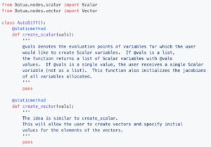
Using the create_scalar and create_vector methods, users are able to initialize variables for use in constructing arbitrary functions. Additionally, users are able to specify initial values for these variables. Creating variables
in this way will ensure that users are able to use the Dotua defined operators to both evaluate functions and compute their derivatives.
Variable Universes
The implementaiton of the AutoDiff library makes the following assumption: for each environment in which the user uses autodifferentiable variables (i.e., Scalar and Vector objects), the user initializes all such variables with a single call to create_scalar or create_vector. This assumption allows Scalar and Vector objects to fully initialize their jacobians before being used by the user. This greatly reduces implementation complexity.
This design choice should not restrict users in their construction of arbitrary functions for the reason that in order to define a function, the user must know how many primitive scalar variables they need to use in advance. Realize that this does not mean that a user is prevented from defining new Python variables as functions of previously created Scalar objects, but only that a user, in defining a mathematical function f(x, y, z) must initialize x, y, and z with a single call to create_scalar. It is perfectly acceptable that in the definition of f(x, y, z) a Python variable such as a = x + y is created. The user is guaranteed that a.eval() and a.partial(x), a.partial(y), and a.partial(z) are all well defined and correct because a in this case is an instance of Scalar; however, it is not a “source” scalar variable and thus the user could not take a partial derivative with respect to a.
rAutoDiff Initializer
The rAutoDiff class functions as an rScalar factory, allowing the user to initialize variables for the sake of constructing arbitrary functions of which they want to later determine the derivative using reverse mode automatic differentiation. Because the same rScalar variables can be used to define multiple functions, users must instantiate an rAutoDiff object to manage the rScalar objects they create and calculate the gradients of different functions of the same variables. Thus, we define the rAutoDiff class in the following way:
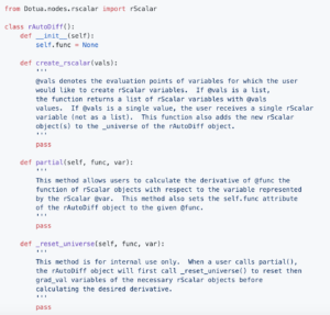
By instantiating an rAutoDiff object and using the create_rscalar method, users are able to initialize variables for use in constructing arbitrary functions. Additionally, users are able to specify initial values for these variables. Creating variables in this way will ensure that users are able to use the Dotua defined operators to both evaluate functions and compute their derivatives. Furthermore, using the partial method, users are able to determine the derivative of their constructed function with respect to a specified rScalar variable.
Operator
The Operator class defines static methods for elementary mathematical functions and operators (specifically those that cannot be overloaded in the Scalar and Vector classes) that can be called by users in constructing arbitrary functions. The Operator class will import the Nodes module in order to return new Scalar or Vector variables as appropriate. The design of the Operator class is as follows:
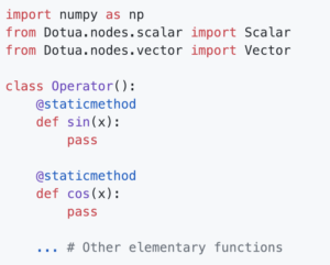
For each method defined in the Operator class, our implementation uses ducktyping to return the necessary object. If user passes a Scalar object to one of the methods then a new Scalar object is returned to the user with the correct value and jacobian. If user passes a Vector object to one of the methods then a new Vector object is returned to the user with the correct value and jacobian. On the other hand, if the user passes a Python numeric type, then the method returns the evaluation of the corresponding NumPy method on the given argument (e.g., op.sin(1) = np.sin(1)).
rOperator
Similarly, the rOperator class defines static methods for elementary mathematical functions and operators (specifically those that cannot be overloaded in the rScalar class) that can be called by users in constructing arbitrary functions. The design of the rOperator class is as follows:
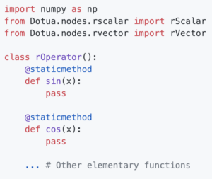
Once again, for each method defined in the rOperator class, our implementation uses ducktyping to return the necessary object. If user passes an rScalar object to one of the methods, then a new rScalar object is returned to the user with the correct value and self/child link. If user passes an rVector object to one of the methods, then a new rVector object is returned to the user
with the correct value and parent/child links. On the other hand, if the user passes a Python numeric type, then the method returns the evaluation of the corresponding NumPy method on the given argument (e.g., rop.sin(1) = np.sin(1)).
A Note on Comparisons
It is important to note that the Dotua library intentionally does not overload comparison operators for its variables class (i.e., Scalar, rScalar, Vector, and rVector). Users should only use the the equality and inequality operators == and != to determine object equivalence. For users wishing to perform comparisons on the values of functions or variables composed of Scalar, rScalar, Vector, or rVector variables with the values of functions or variables of the same type, they can do so by accessing the values with the eval() function.
External Dependencies
Dotua restricts dependencies on third-party libraries to the necessary minimum. Thus, the only external dependencies are NumPy, and SciPy NumPy is used as necessary within the library for mathematical computation (e.g., trigonometric functions). SciPy is used within the Newton-Raphson Demo as a comparison.
Demos
We demonstrated two use-cases for our Python library. The first was using Newton’s method to find the minimum of a convex function, and the second was doing gradient descent to update the weights of a neural network.
Newton’s Method
Newton’s method is a classic way to find the roots of a function. It can be cast into an optimization technique for a differentiable function, where we are solving for the roots of the first derivative. The algorithm begins at an initial point in the domain of the function, and iteratively approximates the minimum through the following update function:

In action, our library runs this algorithm to find the minimum of a quadratic function as follows:


Neural Network
For some output y_hat and set of inputs X, the task of a neural network is to find a function which minimizes a loss function, like MSE:
Where N is the number of data points, yhat_i the value returned by the model and y_i the true value for y at a given observation i. A neural network typically has multiple layers of nodes connected by a web of edges, each with a weight value. The task is to find the weights that minimize the distance between y_hat and y. This is computationally burdensome. Reverse AD is a particularly useful means of traversing the graph and refitting those weights.
We implemented a toy neural network that has only one hidden layer. Using R.A. Fischer’s well-known Iris dataset — a collection of measurements of flowers and their respective species — we predict species based on their floral measurements.
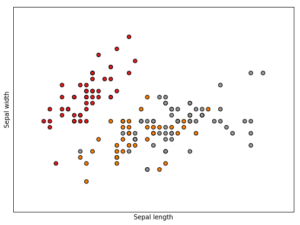
As the scatter plot indicates, there is a clear separation boundary between the setosa plants and the other two species, versicolor and virginica. Our simple network’s performance is summarized in the confusion matrix below:
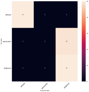
To capture the boundary between each species would require more complexity, and so our simple neural network can only capture the biggest boundary — a consequence of our package using reverse auto differentiation to fit the appropriate gradient. However, this is just an illustration of one very useful application.